Here is a bunch of brief informal impressions on the ideas behind some of the reinforcement learning papers I enjoyed at NeurIPS 2020. For the full story, including the experimental or theoretical results, I encourage you to check out the full works, that are linked. The common thread in all of these works? Some form of, explicit or implicit, model-based reinforcement learning.

• Value-driven Hindsight Modelling
• The Value Equivalence Principle for Model-Based Reinforcement Learning
• Forethought and Hindsight in Credit Assignment
• Self-Paced Deep Reinforcement Learning
• Emergent Complexity and Zero-shot Transfer via Unsupervised Environment Design
• Discovering Reinforcement Learning Algorithms
• Novelty Search in Representational Space for Sample Efficient Exploration

Value-driven Hindsight Modelling

Learning a value function is perhaps one of the most important subproblems to be solved inside many reinforcement learning algorithms. Despite being well-studied, it remains quite hard in many contexts, for a number of reasons. One of these reasons, according to the study of Value-driven Hindsight Modelling (ViMO; Guez et al., 2020), is the fact that the signal usually employed for learning a value function approximation is not that good.

Think of it: the world, with its evolution from a state to another, can be extremely complex and rich in information. But then, we learn the value function by just regressing against a scalar target that only depends on the reward function. In some sense, applying the reward function to a state strips away potentially useful information for value function learning. Is there a way to get that information back?

ViMO uses general value functions to augment the value with the information provided by the states subsequent to the one we want to evaluate. It defines two special value function approximators:

$$ \begin{aligned} \underbrace{v^+(s_t, s_{t+1}, \dots, s_{t+k}; \theta)}_{\mathrm{Hindsight\,Value}} &= \psi_{\theta_1}(s_t, \phi_{\theta_2}(s_{t+1}, \dots, s_{t+k})) \\ \underbrace{v^m(s_t; \eta)}_{\mathrm{Model-based\,Value}} &= \psi_{\eta_1}(s_t, \phi_{\eta_2}(s_t)) \end{aligned}$$

Using the hindsight value, a representation \( \phi_{\theta_2} \) of the future states allows to use additional information from the world during learning. Clearly, this kind of approximation cannot be used online, since the future is not available at a given time. A solution is to be model-based, and to learn a representation \( \phi_{\eta_2} \), which only depends on the current state, as a proxy for the one of an entire trajectory of states. It is an uncommon way to be model-based, that usually implies the use of an estimated model of the dynamics for generating imaginary states, but the term is still appropriate.

The three components, the hindsight value, the model-based value and the model \( \phi \) itself are learned in HiMO with three distinct losses and clever gradient stoppings during training. A recurrent neural network can be used to deal with partial observability.

The Value Equivalence Principle for Model-Based Reinforcement Learning

Model-based reinforcement learning methods are recently getting momentum, mainly for their promise of sample efficiency. For years, the standard approach in model learning has been completely agnostic of the downstream task. Recently, the desire to have decision-aware (or control-oriented) models of the dynamics is rising, anticipated by the development of new architectures (e.g., the Predictron; Silver et al., 2016) but mostly initiated by explicit work on value-aware model learning (VAML; Farahamand et al., 2018): the model learned by maximum likelihood estimation is not always the best one, depending on the overall algorithm that is being employed.

VAML and similar works, including my thesis on gradient-aware models (D’Oro et al., 2019), are mostly concerned with the development of new algorithmic solutions to learn models that are more effective for control. But the theoretical understanding of when and how this kind of models are better than the traditional ones is still in its infancy. The study of The Value Equivalence Principle for Model-Based Reinforcement Learning (Grimm et al., 2020) aims at giving some insights on this.

What does it mean for a model to be good for the downstream control task? Well, if we are going to use that model inside the Bellman operator \( \tilde{\mathcal{T}}_\pi \), for a given policy \( \pi \), then a good model is one that guarantees that:

$$ \mathcal{T}_\pi v = \tilde{\mathcal{T}}_\pi v, $$

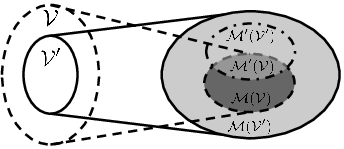
for each policy \( \pi \) in the space of possible policies \( \Pi \) and each value function \( v\) in the space of possible value functions \( \mathcal V \). In other words, a good model is one under which the Bellman operator behaves exactly as the original one. This model is operationally perfect: it does not matter if it is an estimated one, as long as this property is holds. We can thus define, fixed a space of policies and a space of value functions, a whole set of models \( \mathcal{M}(\Pi, \mathcal V) \) that are value-equivalent to the real one \( m^* \), taken from a generic set of models \( \mathcal M \). This set enjoys interesting properties, including:

1. \( \mathcal M’ \subseteq \mathcal M \implies \mathcal M’ (\Pi, \mathcal V) \subseteq \mathcal M (\Pi, \mathcal V)\): having fewer models means having fewer value-equivalent models;
2. \( ( \Pi’ \subseteq \Pi \wedge \mathcal{V}’ \subseteq \mathcal{V}) \implies \mathcal M (\Pi, \mathcal{V}) \subseteq \mathcal{M} (\Pi’, \mathcal{V}') \): having fewer policies and value functions means having more value-equivalent models;
3. \( m^* \in \mathcal M \implies m^* \in \mathcal M (\Pi, \mathcal V), \,\, \forall \Pi \, \forall \mathcal V \): the real model is always value-equivalent to itself.

An interesting fact is that is often possible to represent \( \Pi \) and \( \mathcal V \) as the span of smaller sets of policies and value functions and still keeping the value-equivalence properties of the original sets intact.

Importantly, one can devise a loss function for model learning that is directly inspired by the concept of value equivalence:

$$ \ell_{\Pi, \mathcal V}(m^*, \tilde m) \sum_{\pi \in \Pi, v \in \mathcal V} \| \mathcal T_\pi v - \tilde{\mathcal{T}}v \|, $$

and minimize it on samples.

Existing approaches (like the mentioned Predictron) can be interepreted under the lens of the value-equivalence principle, by varying the form of the Bellman operator and the two sets of policies and value functions.

Forethought and Hindsight in Credit Assignment

One of the most crucial questions in model-based reinforcement is which type of model to use. The standard type of estimated model of the dynamics allows to sample, given a state \( s_t \) and an action \( a_t \), a possible next state \( s_{t+1} \). This kind of model, that has a form of the type \( p(s_{t+1}|s_t, a_t) \), can be called a forward model. The alternative is a so-called backward model, which, instead of predicting the future given the present, predicts the past given the present, and has a form of the type \( p(s_{t-1}, a_{t-1} | s_t) \).

The distinction between forward and backward models is the one between Forethought and Hindsight in Credit Assignment (Chelu et al., 2020). In pratice, there are contexts in which backward planning is more convenient than forward planning and viceversa. It generally depends on the structure of the problem, but there is a crucial hint that could inform us on whether a given Markov Decision Process is more amenable to one type of planning or the other one. In summary, a state has a large fan-in if the agent can end up in it from many states, and a large fan-out if the agent can end up in many states from it: if many states have a large fan-in (channelling is common), then backward planning is more convenient; if many states have a large fan-out (broadcasting is common), then forward planning is more convenient.

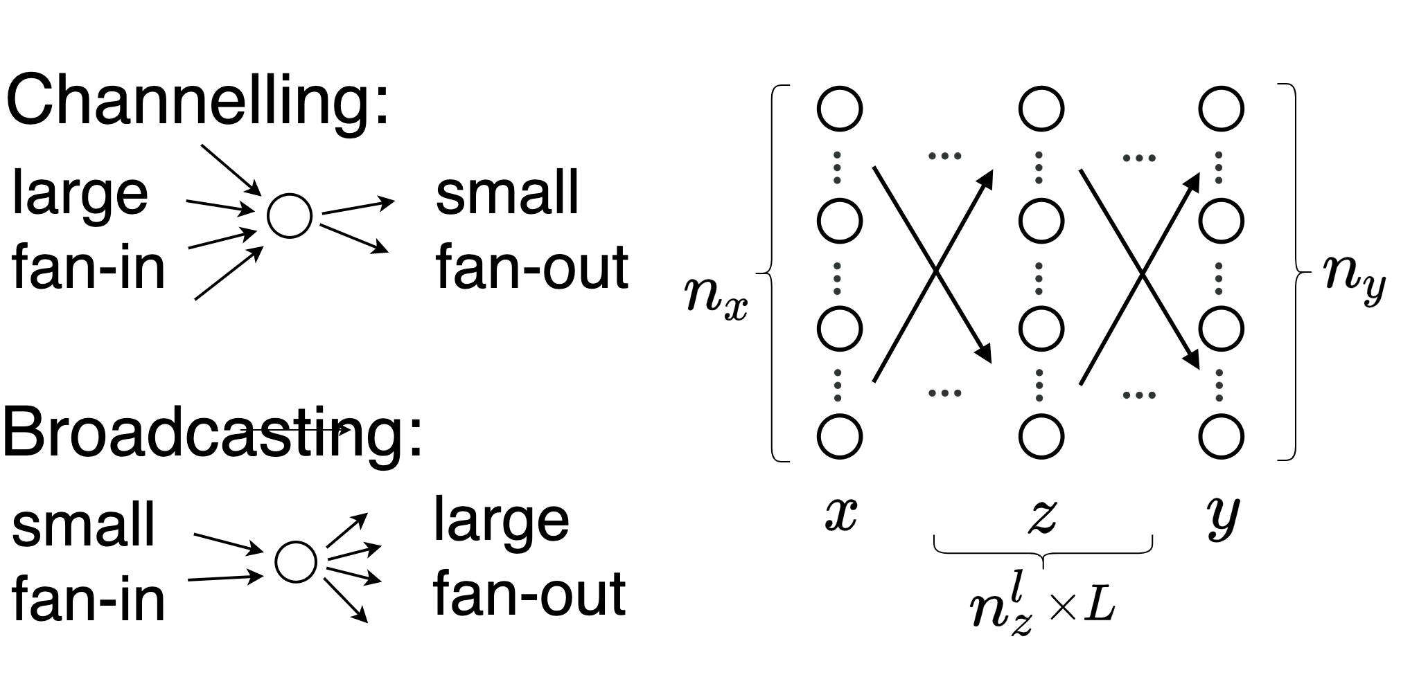
This is pretty intuitive, since the use of a model in place of the real world is more convenient when the observed transitions are not enough representative of the possible ones.

Also in this case, you can ask yourself the question of how to learn such a model, and some hints about it are contained in the paper together with a nice experimental comparison between the two types of models.

Self-Paced Deep Reinforcement Learning

Curriculum learning can be described as the problem of designing a curriculum of tasks that improves the overall training performance of a system. This is a very important open problem in reinforcement learning, in which the agent has much more freedom than the one allowed, for instance, in the supervised learning setting.

In Self-Paced Reinforcement Learning (SPDL; Klink et al., 2020), the agent is allowed to build its own curriculum of tasks in a way that improves its training. A task can be represented by some task vector \( c \), which influences both the reward function \( r_c \) and the transition kernel \( p_c \) of a Markov Decision Process. The overall thing is usually called Contextual Markov Decision Process. Given a distribution over tasks \( \mu(c) \) and a policy \( \pi \), the performance of the agent can be measured by the following objective:

$$ J(\mu, \pi) = \mathbb{E}_{c \sim \mu, p_\pi(\tau|c)} \left[ \sum_{t \geq 0} \gamma^t r_c (s_t, a_t) \right] = \mathbb{E}_{c \sim \mu, p_{0,c}} \left[ V_\omega (s_0, c) \right] = J(\mu, \omega), $$

where \( p_\pi(\tau|c) \) is the distribution of the trajectories of states induced by the given policy and task, and \( p_{0,c} \) is the initial state distribution due to a task.

A clever idea to automate the creation of a curriculum is to let the agent select by itself the pace of its training, by learning a parameterized distribution over tasks \( p_\nu \) and maximizing the performance under the tasks sampled from it. With no constraints, the agent would select the easiest tasks around, with no hope to perform well under the original task distribution \( \mu(c) \). The solution is to constrain \( p_\nu \) to be not-so-far from the real one, and also to move the learned distribution in a rather slow way across iterations. Overall, this is the update rule for the task parameters:

$$ \max_{\nu_{i+1}} \frac{1}{K} \sum_{k=1}^K \frac{p_{\nu_{i+1}}\left(c^k\right)}{p_{\nu_i}\left(c^k\right)} V_{\omega_{i+1}}\left(s^k_0, c^k\right) {-} \alpha_i D_{KL}(p_{\nu_{i+1}}(c)||\mu(c)) \\ \text{s.t.}\ D_{KL}(p_{\nu_{i+1}}(c)||p_{\nu_i}(c)) {\leq} \epsilon, $$

which can be performed in an alternate way with the traditional update of the value function parameters \( \omega \) given a fixed task vector sampled as in \( c \sim p_\nu \). Note that the first term is the importance-weighted approximation for \( J \).

The resulting algorithm can be interpreted as an instance of control as inference.

Emergent Complexity and Zero-shot Transfer via Unsupervised Environment Design

A setting that is related to Contextual Markov Decision Processes is the one in which additional parameters \( \theta \) can be picked to determine the actual dynamics of the environment \( p_\theta(s_{t+1}|s_t, a_t) \). This is called an underspecified Markov Decision Process in Emergent Complexity and Zero-shot Transfer via Unsupervised Environment Design (UED; Dennis et al., 2020), but was explored in the past under the name of Configurable Markov Decision Process.

The possibility of changing some aspects of the underlying dynamics allows, once again, the automated construction of a curriculum. We can follow an idea that is somehow opposite to the one of SPDL: iteratively, an entity, let’s call it the adversary, can optimize the configuration of the MDP in order to produce the most difficult dynamics possible, and the agent, let’s rename it as the protagonist, can perform as good as possible inside the environment with this nasty dynamics. A fundamental problem with this approach is that, in many cases, it would be easy for the adversary to craft an environment that completely blocks the agent in its actions and makes solving the task completely impossible.

The solution is to introduce a third character, the antagonist. If we name \( \pi^P \) the protagonist, \( \pi^A \) the antagonist and \( U^\theta \) their return collected inside the MDP with parameters \( \theta \) picked by the adversary, we can define a form of regret as:

$$ R^\theta(\pi^P, \pi^A) = U^\theta(\pi^A) - U^\theta(\pi^P). $$

Then, the updates for adversary, antagonist and protagonist can be the following, interleaved with the collection of new data from the ever-changing environment:

• \( \max_\theta R^\theta(\pi^P, \pi^A) \)
• \( \max_{\pi^A} R^\theta(\pi^P, \pi^A) \)
• \( \min_{\pi^P} R^\theta(\pi^P, \pi^A) \)

That is, the adversary and the antagonist try to maximize the regret, while the protagonist tries to minimize it. In this way, the adversary cannot trivially make the task impossible for every possible policy, because it would otherwise become impossible also for the antagonist. Instead, it will try to find tasks that are interesting enough to be solvable by the antagonist but hard enough to be challenging for the protagonist, naturally leading to a curriculum.

Discovering Reinforcement Learning Algorithms

Many researchers (including me) believe meta-learning is one of the key ingredients that are leading us to a new generation of very efficient algorithms. But what are the limits of the things that we can meta-learn?

In Discovering Reinforcement Learning Algorithms (Oh et al., 2020), these limits are really pushed in RL. The goal is to let the algorithm discover both a mechanism for policy update and a mechanism possibly similar to bootstrapping. This discovery can be carried out by acting in different environments and then generalized to new environments.

The agent is required to output two probability distributions:

• A policy \( \pi_\theta (a|s) \), which, as usual, is a probability distribution over actions given a state
• A prediction vector \( y_\theta(s) \), which is instrumental to the improvement of the agent.

In a way, this is the standard two-headed architecture used in many actor-critic algorithms: \( y_\theta \) indeed converges after training to something similar to the real value function.

The meta-learner, or Learned Policy Gradient (LPG), is an LSTM that takes as input the sequence of \( x_t = ( r_t, d_t, \pi (a_t|s_t), y_\theta (s_t), y_\theta(s_{t+1}) ) \), the reward, the done condition, the action probability (which makes the algorithm agnostic of the state and the action dimensionalities) and the predictions. The LPG is trained to output two hyperparameters \( \eta = (\widehat A, \widehat y ) \), used in the policy update, which is governed by this law:

$$ \Delta \theta \propto \mathbb{E}_\theta \left[ \nabla_\theta \log \pi_\theta (a | s)\widehat A - \alpha \nabla_\theta D_{KL} (y_\theta(s) || \widehat y) \right], $$

where \( \widehat A \) is used exactly as the advantage or the return in likelihood ratio policy gradient methods.

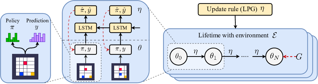
The hyperparameters \( \eta \) are then updated by likelihood ratio methods to maximize the actual return \( G \) observed in the environment:

$$ \Delta \eta \propto \mathbb{E}_{\theta_{N-k}} \left[ \nabla_\eta \log \pi_{\theta_N}(a|s) G \right]. $$

Thus, the algorithm backpropagates through the update process that lead from \( \theta_{N-k} \) to \( \theta_N \). Heavy regularization schemes are then necessary to stabilize the training.

The objective for hyperparameters learning is computed across environments and tasks: the learned update rule can then be used in much complex tasks (e.g., learning the update rule on toy problems and employing it for the ATARI games).

Novelty Search in Representational Space for Sample Efficient Exploration

The quest for effective exploration methods is one of the most important ones in reinforcement learning. It is deeply entangled with the problem of representation learning, since a good representation is fundamental to determine whether a state of the environment could be interesting or not. The two problems are jointly faced in Novelty Search in Representational Space for Sample Efficient Exploration (Tao et al., 2020), which employs ideas from the most celebrated information-theoretic formulation of representation learning, the information bottleneck (Thishby et al., 2000).

The exploration strategy presented in the paper is a graph-theoretic one, based on novelty search. If the representation of a state \( s \in \mathcal{S} \) is given by a smaller vector \( x \in \mathcal{X} \), then the states previously encountered by the agent will be points in \( \mathcal{X} \) with a certain distance the one from the other. We can obtain a measure of the sparsity around \( x \) by considering its \( k\)-nearest neighbors and computing it as:

$$ \widehat \rho_{\mathcal X} (x) = \frac{1}{k} \sum_{i=1}^k d(x, x_i). $$

By using this as an exploration bonus, alongside the task reward, the agent will be curious about the states whose representation is far apart from the one of the familiar states. This is pretty intuitive, but requires the construction of an appropriate representation space \( \mathcal X \).

Here is where the information bottleneck comes in. To learn the representation, it prescribes an optimization problem of the kind:

$$ \min \underbrace{I[S';X']}_{\text{Information shared between} \\ \text{a state and its representation}} - \beta \underbrace{I[X';X,A]}_{\text{Information shared between} \\ \text{a state, an action and the next state}} $$

\( I \) is the mutual information, the information that you can obtain about a random variable by looking at another one. We want the representation to be as informative as possible about the dynamics, the transitions that happen from one state to another, but at the same time throwing away as much of the pointless or distracting content of the state as possible. The latter objective can be achieved by selecting the dimensionality of the representation to be much smaller than the state dimensionality, that is \( \dim( \mathcal X) \ll \dim ( \mathcal S) \). The former one can be achieved by more or less traditional model learning akin to the one of traditional model-based reinforcement learning. Indeed:

$$ I[X';X,A] = H[X'] - H[X' | X, A], $$

so we would like to minimize the entropy \( H \) of the next state distribution given the preceding state and action and maximize the entropy of the representation. The first one is minimized by simple maximum likelihood estimation on the observed transitions; the second one can be maximized by minimizing the expected pairwise Gaussian potential.

The last ingredient for learning an encoding function \( e: \mathcal S \rightarrow \mathcal X \) is some regularization to be sure that a metric such as the euclidean distance behaves well in the resulting space \( \mathcal X \). You can then compute the intrinsic reward \( \widehat \rho_{\mathcal X}\), and also employ the learned dynamics model for planning on top of traditional DQN.