There is a number of potential gains in using an approximate model in reinforcement learning, in terms, for instance, of safety and, as most commonly affirmed, sample-efficiency. However, there is an advantage that should not be forgotten and that is, perhaps, the most interesting: approximating the environment dynamics can unlock peculiar learning modalities that would be impossible in a model-free setting. We will see in this blog post that model-based techniques can be leveraged to obtain a critic that is tailor-made for policy optimization in an actor-critic setting. How? By allowing the critic to explicitly learn to produce accurate policy gradients.
Actor-critic methods
A common paradigm in policy gradient reinforcement learning methods is the actor-critic one: an actor \( \pi_{\mathbf{\theta}} \), that determines the control policy for acting in the environment, is improved thanks to a critic \( Q_{\mathbf{\phi}} \), that estimates the cumulative reward of the corresponding actor. For the rest of the post, let’s assume \( \pi \) is deterministically producing actions to act in the environment. In this context, the typical technique used for updating the actor consists in moving its parameters towards the direction that maximizes the value produced by its critic, i.e., its estimated expected return:
considering a state \( s \) collected in the environment. This is a generalization of the basic idea behind Q-learning (i.e., computing \( \max_{a} Q(s,a) \)) to continuous actions spaces, in which the maximization operation cannot be easily performed.
How to learn a good critic?
In the actor-critic framework, any improvement of the actor depends on its critic, so we really would like to have the best possible performance from it. But what does it mean for a critic to be well-performing? Well, the common wisdom is to learn the critic by temporal difference (TD) learning. Defined \( \widehat{\delta}^{\pi_{\mathbf{\theta}}, Q_{\mathbf{\phi}}}(s,a,s’) = r(s,a) + \gamma Q_{\mathbf{\phi}}(s’,\pi_{\mathbf{\theta}}(s’)) - Q_{\mathbf{\phi}}(s,a) \), the bootstrapped deviation of the critic w.r.t. the true value function, this amounts to updating the critic parameters \( \mathbf{\phi} \) by the following step of minimization by gradient descent:
\[\mathbf{\phi} \gets \mathbf{\phi} - \alpha_{Q} \nabla_{\mathbf{\phi}} \left| \widehat{\delta}^{\pi_{\mathbf{\theta}}, Q_{\mathbf{\phi}}}(s,\pi_{\mathbf{\theta}}(s),s') \right|,\]on transitions of the type \( (s,\pi_{\mathbf{\theta}}(s), s’) \) collected in the environment. Did you notice anything uncomfortable? To improve the actor, we would like \( \nabla_a Q_{\mathbf{\phi}} \) to be accurate w.r.t. to the real one (i.e., \( \nabla_a Q_{\mathbf{\phi}} \approx \nabla_a Q^\pi \)). However, in TD-learning we are actually trying to get to the point where \( Q_{\mathbf{\phi}} \approx Q^\pi\). If we could hope to perfectly match, at some point in the optimization problem, our critic with the true value function, with no time, data and approximation limits, this would not be a problem: if a critic is perfect, it is perfect in any sense. Unfortunately, in the policy optimization context, we have many time, data and approximation concerns. We typically have:
- No time to fully evaluate a policy before improving it, thus changing it;
- Not enough data from a given policy to properly evaluate it;
- Finite, even if good, approximation capabilities.
Therefore, we would like to procede straight to the point, and directly learn \( \nabla_a Q_{\mathbf{\phi}} \), what we actually need to improve our policy, regardless of how well we perform in the pure evaluation of the actor, i.e., the prediction of its expected return. We would like to have a critic that is good at improving the actor, not necessarily good at telling how the actor is performing.
With that said, we are willing to match the action-gradient of our critic with the one of the real value function or, using TD-learning, with \( \nabla_a ( r(s,a) + \gamma Q_{\mathbf{\phi}}(s’, \pi(s’)) ) \). Therefore, in the ideal case, we would like to improve the critic in the following way:
\[\mathbf{\phi} \gets \mathbf{\phi} - \alpha_{Q} \nabla_{\mathbf{\phi}} \left\| \nabla_a \widehat{\delta}^{\pi_{\mathbf{\theta}}, Q_{\mathbf{\phi}}}(s,\pi_{\mathbf{\theta}}(s),s') \right\|,\]on transitions collected in the environment. This looks promising, isn’t it? But it is actually highly unpractical.
Computing \( \nabla_a \widehat{\delta}^{\pi_{\mathbf{\theta}}, Q_{\mathbf{\phi}}} \), the action-gradient of the TD-error, requires to have the real environment dynamics at our disposal in a differentiable form. We need, in fact, to compute \( \nabla_a Q_{\mathbf{\phi}}(s’, \pi_{\mathbf{\theta}}(s’))\), to see how the action taken by the agent in a step affects the value at the subsequent step. It is even more clear to see by looking at the computational graph constructed when computing the TD-error.
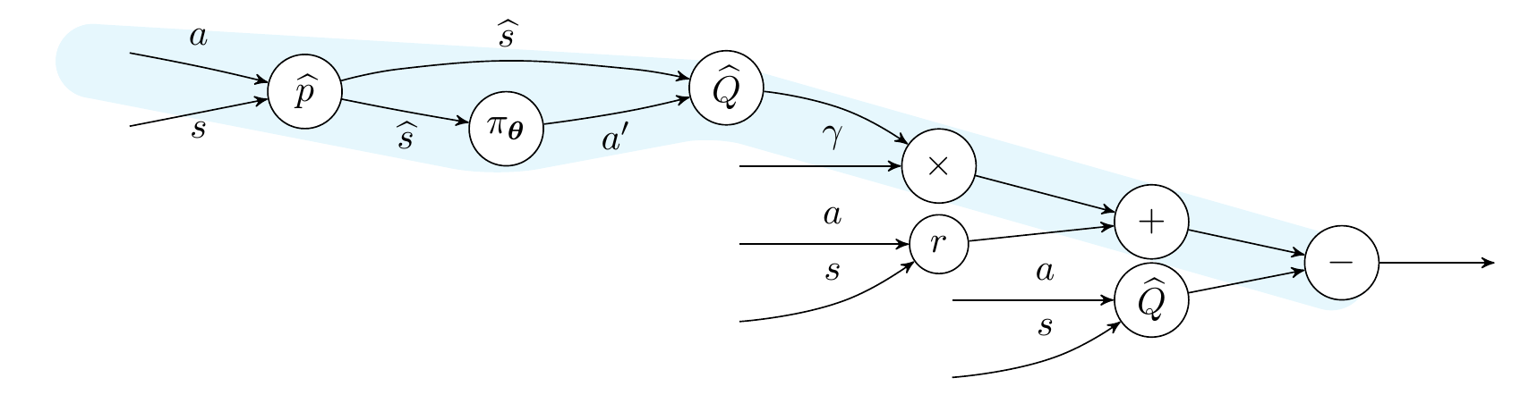
Computational graph of the TD-error
The path in the graph that is highlighted in cyan requires differentiation through the environment dynamics. And guess what? The world is not differentiable, so we must figure out a way to obtain an approximate version of the required gradients.
Making the world differentiable
Recently, there has been a resurgence of model-based reinforcement learning methods. In these approaches, as opposed to the model-free ones, an estimated model of the dynamics of the environment is used for learning a control policy. In the actor-critic setting, we have, therefore, three moving parts that interact and contribute to improving the performance of the agent. We want to learn the approximate model \( p_{\mathbf{\omega}} \) to obtain a better critic \( Q_{\mathbf{\phi}} \) that will improve the actor \( \pi_{\mathbf{\theta}} \).
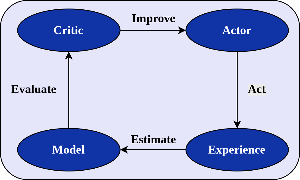
Structure of a model-based actor-critic algorithm
The use of a model can have benefits per-se, but, importantly, if we use a neural network or any other class of differentiable models, it is possible to properly construct the computational graph of the TD-error and, effectively, make the world differentiable. Or, at least, an approximate version of it. We can freely use even stochastic models, by leveraging the reparameterization trick.
This is enough to give a try to the minimization of the proper loss function we talked about. However, it turns out this minimization problem for critic learning is surprisingly hard to solve in practice, prone to degenerate solutions. We should therefore circumvent this issue, before getting to an actual algorithm.
We need a MAGE!
A remedy to avoid degenerate solutions is to constrain the general minimization problem. A natural way to do it? By using the TD-error itself. Formally, we would like to solve the following problem:
\[\min_{\widetilde{\mathbf{\phi}} \in \Phi} \mathop{\mathbb{E}}_{\substack{\text{$s \sim d_\mu^\pi$}\\\text{$\widehat{s} \sim p_{\mathbf{\omega}}(\cdot|s,\pi(s))$}}}\left\| \nabla_a \widehat{\delta}^{\pi, Q_{\widetilde{\mathbf{\phi}}}}(s,a,\widehat{s})\Big|_{a=\pi(s)} \right\| \\ \mathrm{s.t. } \mathop{\mathbb{E}}_{\substack{\text{$s \sim d_\mu^\pi$}\\\text{$\widehat{s} \sim p_{\mathbf{\omega}}(\cdot|s,\pi(s))$}}} \left| \widehat{\delta}^{\pi, Q_{\widetilde{\mathbf{\phi}}}}(s,\pi(s),\widehat{s}) \right| \leq \lambda.\]The cheapest way to approximately solve it is to use penalty function methods, or, simply put, to minimize a linear combination of the traditional TD-error and the error in terms of gradient of critic:
\[\mathbf{\phi} \gets \mathbf{\phi} - \alpha_{Q} \nabla_{\mathbf{\phi}} \left( \left\| \nabla_a \widehat{\delta}^{\pi_{\mathbf{\theta}}, Q_{\mathbf{\phi}}}(s, a, \widehat{s}) \big|_{a=\pi_{\mathbf{\theta}}(s)} \right\| \\ \qquad \, + \lambda \left| \widehat{\delta}^{\pi_{\mathbf{\theta}}, Q_{\mathbf{\phi}}}(s, a, \widehat{s}) \right| \right),\]on transitions \( (s, \pi_{\mathbf{\theta}}, \widehat{s})\) whose next state is sampled from the differentiable approximate model \( p_{\mathbf{\omega}}\).
Learning a critic in this way will produce more accurate gradients, thus improving the actor faster.
We can insert this procedure for critic learning into a fully-fledged Dyna-based algorithm. We iteratively interact with the environment, learn the model, improve the critic with our gradient-tailored loss computed on transitions whose next state is imaginary, and improve the actor by ascending the policy gradient provided by the critic. We call this approach Model-based Action-Gradient Estimator Policy Optimization (MAGE).
Empirical performance of MAGE
In practice, you can use for MAGE any modern deterministic policy gradient algorithm as a base algorithm. For a model-free algorithm, you just need two steps:
- Introduce a learned dynamics model and generate transitions from this model instead of the environment;
- Learn the critic by also minimizing by temporal-difference the error on the action-gradient.
We instantiated MAGE by using TD3 as a base algorithm, alongside an ensemble of Gaussian models.
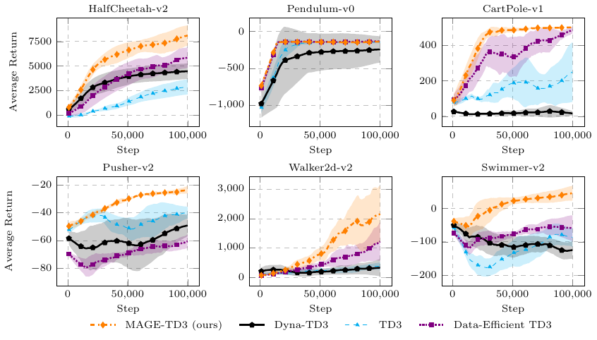
Performance of MAGE on continuous control tasks
In comparison with model-free and model-based baselines, you can see that MAGE is significantly more sample efficient in continuous control tasks. This shows the advantage of directly learning to improve the policy, and not only to evaluate it.
Bonus Observation
The Dyna-TD3 baseline is a modification of MAGE in which only the TD-error is classically minimized for learning the critic, but a model is still used for generating imaginary states. You can see this version is not only worse than MAGE, but also no better than Data-Efficient TD3, a model-free greedy version of TD3. There is a deep meaning in this. Model-based algorithms are not more sample-efficient than model-free algorithms by default. But while determining under which circumstances there is an advantage in the use of a model in an otherwise model-free algorithm is an interesting problem, the sure thing is that using a model can lead you to novel learning modalities, such as the gradient-learning procedure I just described. And this makes model-based reinforcement learning incredibly interesting.
“Archeological” connections
MAGE is backed by relatively recent theoretical work (2014-ish). Nonetheless, the idea of leveraging an approximate model to handle or even learn gradients can be interestingly traced back. The expression “Making the world differentiable”, that I previously used in this post, is a quotation of Jürgen Schmidhuber’s 1990 paper, that also leverages the general idea of employing an approximate model as a proxy for a differentiable environment. An even more incredible connection is with a work originally published by Paul Werbos in 1977, that contains the idea of learning the gradient of a state-value function. Different spirit, motivation (generalization over new trajectories) and framework (deterministic models, no “deep” learning), but an outstanding demonstration of the braveness and topicality of the ideas of the first connectionist era.
Overall, I have a strong feeling that this idea of a deeper connection and interaction between model, critic and actor was strong during that time. It is in a way not surprising, as this is arguably one of the most natural ways to solve a reinforcement learning problem, more akin to classical control theory but at the same time more in line with what is now known as differentiable programming.
This work was carried out at NNAISENSE, together with the amazing Wojciech Jaśkowski. Read our paper or watch our Github repo for more info.