pirandello You recognized it. This is the super-handy expression for the policy gradient derived more than 20 years ago by Richard Sutton and colleagues. In this blog post, I will show how the Policy Gradient Theorem can offer a lens to interpret modern model-based policy search methods. Yes, even the ones that do not directly consider it.

A recap on the Theorem – The Model-Free Gradient

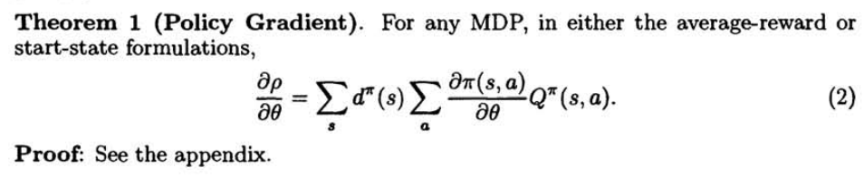
Let’s first state the theorem using a convenient notation¹. Given $ J $, the performance of a stochastic differentiable policy $ \pi_\theta $, the gradient with respect to its parameters is given by:

$$ \nabla_\theta J(\theta) = \int d^{\pi}(s,a) \nabla_\theta \log \pi_\theta(a|s) Q^{\pi}(s,a) \mathrm{d}s \mathrm{d}a.$$

In other words, if you look for an improvement direction for the performance of a policy, you should take three elements into account:

$ d^{\pi}(s,a) $, the stationary distribution of states and actions in the environment if $ \pi $ is executed;
$ \nabla_\theta \log \pi_\theta (a|s) $, the score, linked to the possibility of a change in the parameters of the policy on a given state and action;
$ Q^{\pi}(s,a) $, the expected cumulative discounted return that follows the execution of action $ a $ in state $ s $.

Since the policy is usually available and the chosen policy class is convenient, computing the score is usually not a problem. More delicate is instead the choice of how to handle the other two factors, since they depend on the dynamics of the environment $ p(\cdot | s, a ) $. Indeed, this design choice can determine the type of gradient that you are going to use to improve the policy, with significant consequences.

To see this more clearly, let’s write once again the statement of the Policy Gradient Theorem, making the dependence of the different elements on the environment model $ p $ explicit:

$$ \nabla_\theta J^\mathrm{MFG}(\theta) = \int d^{\pi,p}(s,a) \nabla_\theta \log \pi_\theta(a|s) Q^{\pi,p}(s,a) \mathrm{d}s \mathrm{d}a,$$

where the acronym MFG stands for Model-Free Gradient, to highlight the fact that only the dynamics from the environment is considered in it. To sample from $ d^{\pi,p} $ and estimate $ Q^{\pi,p} $, one can query the model $ p $, i.e., interact with the real environment: this is at the core of any, old or new, model-free policy gradient algorithm based on stochastic policies. For instance, by sampling states and actions along trajectories generated by $ \pi $ and using the empirical return of the trajectory as a proxy for the true value, you obtain the classical REINFORCE estimator.

However, interacting with the environment can be costly, and estimating the gradient from samples in this fashion can easily yield high variance.

The common alternative: the Fully-Model-based Gradient

One of the biggest promises of model-based reinforcement learning is to increase sample efficiency: to reduce the variance at the cost of introducing a bias. The source for the bias is the use of an estimated model $\widehat{p}(\cdot | s,a) $, that can substitute the real model when needed.

In policy gradient approaches, this translates into a $ p \leftrightarrow \widehat{p} $ substitution inside the two quantities that appear in the Policy Gradient Theorem. The most common way to inject an estimated model into an approximation for the policy gradient leads to the following definition:

$$ \nabla_\theta J^\mathrm{FMG}(\theta) = \int d^{\pi,\widehat{p}}(s,a) \nabla_\theta \log \pi_\theta(a|s) Q^{\pi,\widehat{p}}(s,a) \mathrm{d}s \mathrm{d}a,$$

that we can call Fully Model-based Gradient, FMG for short. This is an approximation for the policy gradient: on the one hand, this is a different quantity than the true policy gradient as prescribed by the theorem; on the other hand, an appropriately accurate estimate of the dynamics will yield a gradient that is pretty close to the true one, at the same time with all the advantages of having an estimated model in you hands.

Using an FMG simply amounts to substituting the real environment with a learned simulator, a world model $ \widehat{p} $. If you run any standard model-free policy gradient algorithm using a $ p \leftrightarrow \widehat{p} $ substitution, you are either implicitly or explicitly using this approximation. Of course, you can leverage a learned model in additional ways², but the approach is undoubtedly simple on a conceptual level.

If the model is extremely good, then the FMG is effective for improving the policy; however, the environment can be really complex, and the risk of introducing high bias due to a faulty model is high.

Understanding the less common alternative: the Model-Value-based Gradient

A natural question that arises on the use of an estimated model is whether its bias effect can be reduced, still leveraging its expressive power in order to get an improvement over standard model-free approaches.

An answer to this question can be extracted by a slight, yet significant, modification to the formulation given by the Policy Gradient Theorem. This yields a new approximation:

$$ \nabla_\theta J^\mathrm{MVG}(\theta) = \int d^{\pi,p}(s,a) \nabla_\theta \log \pi_\theta(a|s) Q^{\pi,\widehat{p}}(s,a) \mathrm{d}s \mathrm{d}a.$$

We can call it the Model-Value-based Gradient (or MVG): $ \hat{p} $ is only used in the computation of the action-value function $ Q^{\pi} $, but not as an ingredient in crafting the distribution $ d^\pi $ of states and actions. Although it could be seen as a pointless mathematical gimmick, this peculiar use of an estimated model has been used (sporadically) for years in the reinforcement learning community. The presentation in the form offered by the Policy Gradient Theorem sheds some new light on these approaches: learning about the dynamics of the environment is only leveraged for solving credit assignment on existing transitions generated in the real environment. Thus, the effect of the error introduced by the model is mitigated, at the same time retaining a significant part of its representation capabilities.

There is also a more practical perspective on why using the MVG can be a good idea. Since at the moment of estimation of the actual gradient you sample from $ d^{\pi, p} $, the policy and the value function are only queried for data obtained by real interaction with the environment, possibly mitigating an explosion in the error due to out-of-distribution evaluations.

While the design of approaches centered around the Fully-Model-based Gradient can be straightforward, in which cases are you employing the MVG in your algorithm? Remember, the only requirement is, in a policy gradient method, to be using at the same time trajectories generated in the real environment but a value function valid under the estimated model. I will now list three different ways this fact can be present in an algorithm, differing mainly by the way you represent and handle $ Q^{\pi, \widehat{p}} $:

Computation of $ Q^{\pi, \widehat{p}} $ by approximate dynamic programming. A function approximator $ \widehat{Q} $ is used for representing the value function and trained using transitions generated using $ \widehat{p} $. Then, $ \widehat{Q} $ is used along with real states and actions for computing an improvement direction. The approach is used, for instance, in MBPO (Janner et al. 2019), when an unrolling horizon of $ k=1$ is used in their model-based version of SAC. The authors report a little bit of aura of mystery around the great empirical effectiveness of the use of $ k=1$, but indeed a valid explanation could be their implicit use of the MVG;
On-the-fly $ Q^{\pi, \widehat{p}} $ Monte-Carlo estimation. There is no explicit representation for the Q-function, that is computed by rolling out the model and computing the total reward, every time there is a need to evaluate $ Q^{\pi, \widehat{p}} $. This method, used in our recent work (D’Oro et al. 2020), allows to overcome the difficulties of TD-learning with function approximation, although it can be computationally demanding;
Backpropagation through real trajectories. Again, no explicit representation for the Q-function is employed. Instead, the estimated model $ \widehat{p} $ is used in the computation of the gradient of the expected return via backpropagation through time (i.e., the value gradient), on data that have been collected in the environment. No unrolling of any kind is done with the estimated model: it is only used for dealing with credit assignment. The method was introduced in its modern version by (Heess et al. 2015), although no explicit reference to MVG-like approximations was made.

It is possible that other powerful methods for handling an MVG can be designed, outside of the umbrella defined by the three techniques just described.

Which type of gradient should you use?

Throughout the blog post, I briefly mentioned some of the relative advantages of the MFG, the FMG and the MVG, in a quite high-level perspective concerning bias and variance. However, providing a precise quantification and a method for deciding which type of gradient is the right one for a given environment or circumstance is still an unexplored problem. Indeed, I honestly believe one of the most important open research question in model-based reinforcement learning concerns understanding under which conditions it’s worthful to leverage a model in a certain way, or even to employ a model at all.

Intuitively, the most important fact to consider when facing these decisions is how good the estimated model $ \widehat{p} $ is. If $ p \approx \widehat{p} $, then the $ p \leftrightarrow \widehat{p} $ substitution operated in the Fully Model-based Gradient does no harm and only unlocks new powerful possibilities. On the other hand, if the estimated model $ \widehat{p} $ is extremely bad, then there is no benefit at all in using it for estimating the gradient, neither through $ d^{\pi,\widehat{p}} $ nor through $ Q^{\pi, \widehat{p}} $, and the Model-Free Gradient should be preferred. The Model-Value-based gradient can be instead a nice alternative when it’s really hard to perfectly model the complete dynamics, but still many useful bits can be captured by $ \widehat{p} $. As a marginal yet interesting point, the use of the MVG can allows some interesting theoretical analyses³, leading to better definitions of the concepts of “good model” and “bad model” in reinforcement learning.

To have a glimpse of many existing policy search approaches can be classified according to this perspective based on the Policy Gradient Theorem, here is a table containing a bunch of (arbitrary) per-category examples.

Model-Free Gradient	Fully Model-based Gradient	Model-Value-based Gradient
REINFORCE (Williams. 1992)	PILCO (Deisenroth et al. 2011)	UIM (Abbel et al. 2016)
TRPO (Schulman et al. 2015)	ME-TRPO (Kurutach et al. 2018)	MBPO (k=1) (Janner et al. 2019)
SAC (Haarnoja et al. 2018)	MBPG (Wang et al. 2003)	SVG (Heess et al. 2015)
POIS (Metelli et al. 2018)	SLBO (Luo et al. 2018)	GAMPS (D’Oro et al. 2020)

Conclusion

Model-based and policy gradient approaches are among the most promising families of reinforcement learning methods currently investigated by the research community. In this post, I outlined a perspective that can be useful to understand how their combination occurred in previous algorithms and maybe offer some inspiration for future research.

I want to thank all the people that discussed this topic with me, at Politecnico di Milano and NNAISENSE.

I’ll be particularly easy on notation (e.g., omitting some normalization constants). ↩
Like backpropagating through the model à la PILCO. ↩
As shown in our paper (D’Oro et al. 2020) and in my Master Thesis. ↩